Post-process parameters#
This tutorial shows how we can use methods available in the Synthetic class to estimate for a given observed cluster:
the individual stellar masses
the per-star probability of being a binary system
the per-star probability of being a blue straggler (BSS)
the initial, actual and fractions of lost mass associated to the cluster
and from the two arrays of probabilities, obtain for the observed cluster:
the total binary fraction
the total number ob BSSs
These processes are described in Synthetic module.
We start by loading the cluster file and a set of isochrones, and instantiating a synthetic object which we calibrate with the cluster’s data:
Instantiating cluster from data
Columns read   : ra, dec, mag, e_mag, color, e_color
N_stars        : 1428
N_clust_min    : 25
N_clust_max    : 2000
Cluster object generated

Instantiating isochrones
Model          : PARSEC
N_files        : 1
N_mets         : 5
N_ages         : 13
N_points       : 2000
z    range     : [0.01, 0.03]
loga range     : [7.0, 10.0]
Magnitude      : Gmag
Color          : G_BPmag-G_RPmag
Isochrone object generated

Instantiating synthetic
Default params : {'met': 0.0152, 'loga': 8.0, 'alpha': 0.09, 'beta': 0.94, 'Rv': 3.1, 'DR': 0.0, 'Av': 0.2, 'dm': 9.0}
Extinction law : GAIADR3
Diff reddening : uniform
IMF            : chabrier_2014
Max init mass  : 10000
Gamma dist     : D&K
Random seed    : 457304
Synthetic clusters object generated

Calibrated observed cluster
N_stars_obs    : 1428
Max magnitude  : 18.99
Error distribution loaded
For all three analyses mentioned above, the first step is to call the get_models() method. This method requires two arguments: model which is a dictionary of parameters to be fitted and a model_std dictionary which contains the uncertainties (standard deviations) associated to each parameter in the model dictionary. For example:
# Values for the fundamental parameters associated to the observed cluster.
# These can be obtained via cluster parameters fitting or set manually
model = {
    "loga": 8.0,
    "dm": 8.17,
    "Av": 0.44,
}
# Uncertainties for each fundamental parameter
model_std = {
    "loga": 0.04,
    "dm": 0.04,
    "Av": 0.03,
}

# Call the method
synthcl.get_models(model, model_std)
Generate synthetic models
N_models       : 200
Attributes stored in Synthetic object
This method will store in the synthcl object a number of synthetic clusters, sampled from a normal distribution centered on model values with STDDEVs taken from the model_std values.
After calling this method, the cluster mass, individual stellar masses and binary system and BSSs probabilities can be estimated as shown in the following sub-sections.
Stellar masses and probabilities#
To assign individual primary and secondary masses and probability of belonging to a binary system for each observed star in your cluster, we use the the stellar_masses() method:
stellar_data = synthcl.stellar_parameters()
Stellar masses and binary+BSS probabilities estimated
/home/gabriel/Github/ASteCA/ASteCA/asteca/asteca/synthetic.py:581: UserWarning:
N=9 stars found with no valid photometric data. These will be assigned 'nan' values
for masses and binarity probability
  warnings.warn(
The warning indicates that some observed stars contain invalid photometric data and thus could not be assigned masses.
The returned variable stellar_data is a dictionary containing the columns m1, m1_std, m2, m2_std, binar_prob, bss_prob. We can print the resulting dictionary as a pandas DataFrame for better visualization:
# As pandas DataFrame for prettier printing
stellar_data = pd.DataFrame(stellar_data)
stellar_data
| m1 | m1_std | m2 | m2_std | binar_prob | bss_prob | |
|---|---|---|---|---|---|---|
| 0 | 0.532507 | 0.006685 | 0.171730 | 1.904618e-02 | 0.075 | 0.00 |
| 1 | 1.445053 | 0.020363 | 0.236852 | 1.526099e-01 | 0.570 | 0.00 |
| 2 | 1.080898 | 0.015769 | 0.354642 | 1.110223e-16 | 0.075 | 0.00 |
| 3 | 0.792107 | 0.011759 | 0.201585 | 4.146848e-02 | 0.010 | 0.00 |
| 4 | 0.882202 | 0.012553 | NaN | NaN | 0.000 | 0.00 |
| ... | ... | ... | ... | ... | ... | ... |
| 1423 | 4.654422 | 0.166398 | 2.381882 | 1.305031e+00 | 0.890 | 0.95 |
| 1424 | 5.171399 | 0.093816 | 0.106330 | 2.057773e+00 | 1.000 | 1.00 |
| 1425 | 4.654422 | 0.178770 | 1.010461 | 1.457195e+00 | 0.915 | 1.00 |
| 1426 | 4.654422 | 0.179856 | 1.010461 | 1.661577e+00 | 0.920 | 1.00 |
| 1427 | 5.171399 | 0.015368 | 0.106330 | 1.539119e+00 | 1.000 | 1.00 |
1428 rows × 6 columns
These columns represent, for each observed star in the cluster under analysis, estimates for:
m1: primary massm1_std: uncertainty of the primary massm2: secondary mass (under the assumption that this star is part of a binary system)m2_std: uncertainty of the secondary massbinar_prob: probability of being a binary systembss_prob: probability of being a blue straggler
If an observed star has binar_prob=0, i.e. a zero probability of being a binary system, then the mass value for its secondary star m2 is a NaN value as no secondary star could be assigned to it. If any observed star contains invalid photometric data, they will be assigned NaN values for masses and binarity probability.
For example, we can extract the binary systems from the above dictionary by selecting a probability cut at binar_prob=0.5 so that observed stars with larger probability values are described as binary systems. We can visualize the identified single and binary systems in a simple CMD:
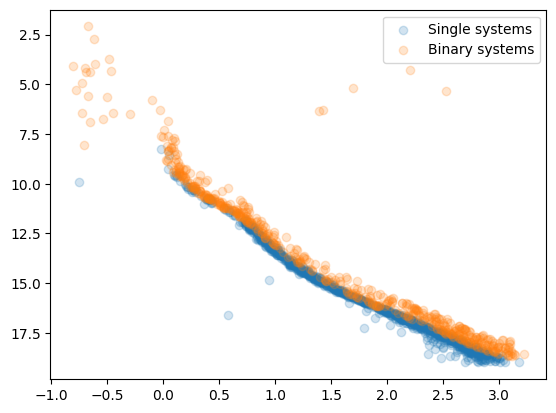
Notice that stars in the BSS region of the CMD (brighter and bluer than the turn-off point) are also identified as very probable binary systems. As explained in Synthetic module, the binary probabilities for BSSs are not accurate and should not be used.
The following section explains how to estimate the cluster’s total binary fraction taking this into account.
Binary fraction#
As detailed in Synthetic module, there is no total binary fraction parameter fitted when using the synthetic clusters, as this is handled through the alpha, beta parameters. The binary fraction parameter can be easily estimated using the probabilities found above, as follows:
# Extract the per-star binary probabilities
binar_probs = stellar_data['binar_prob']

# Exclude nan values (stars with bad photometry)
msk = ~np.isnan(binar_probs)
binar_probs = binar_probs[msk]

# Obtain mean and STDDEV of the total binary fraction for this cluster
bfr_med = np.mean(binar_probs)
# Measure the STDDEV as the standard error of the mean for Bernoulli variables
# (ie: NOT np.std(binar_probs))
bfr_std = np.sqrt(np.sum(binar_probs * (1 - binar_probs))) / len(binar_probs)
print(f"Binary fraction: {bfr_med:.2f}+/-{bfr_std:.2f}")
Binary fraction: 0.36+/-0.01
To get an estimate that is slightly more accurate, we can discard the most probable BSSs (which most likely will have large binary probabilities) before estimating the total binary fraction
# Extract BSS probabilities (without nan values)
bss_probs = stellar_data['bss_prob'][msk]

# Identify those stars that have a probability of being a BSS lower than 50%
msk_bss = bss_probs < 0.5

# Re estimate the meand and STDDEV of the total binary fraction for this cluster,
# now excluding those stars that are most likely BSSs
binar_probs = binar_probs[msk_bss]
bfr_med = np.mean(binar_probs)
bfr_std = np.sqrt(np.sum(binar_probs * (1 - binar_probs))) / len(binar_probs)
print(f"Binary fraction: {bfr_med:.2f}+/-{bfr_std:.2f}")
Binary fraction: 0.35+/-0.01
As we can see, the estimate is a bit smaller as we removed a few probable BSS stars that also have large probabilities of being binary systems.
The following section shows how the total number of BSSs can be estimated.
Number of BSSs#
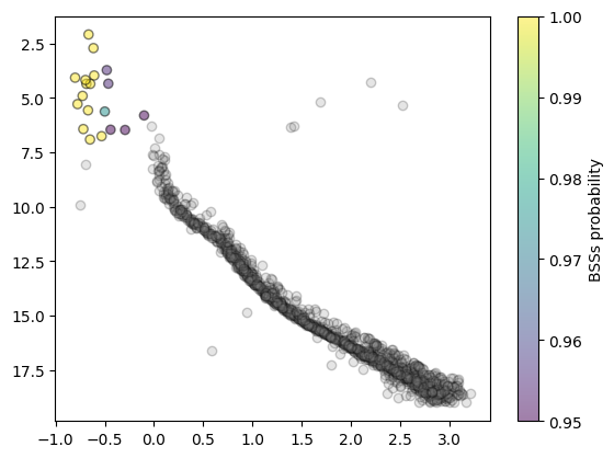
We can obtain the number of detected BSSs using for example a probability cut of P=50%:
# Extract BSS probabilities
bss_probs = stellar_data['bss_prob']

# Identify as BSSs only those stars with probabilities larger tan 50%
msk_bss = bss_probs > 0.5

# Count BSSs
N_bss = msk_bss.sum()
print(f"Number of BSSs detected: {N_bss}")
Number of BSSs detected: 19
A simple plot shows which observed stars are more likely to be BSSs:
Mass(es) estimation#
As explained in the Cluster mass section, ASteCA estimates several different masses associated to an observed cluster. These are:
\(M_{init}\): total initial mass (at the moment of cluster’s birth)
\(M_{actual}\): actual mass of the cluster (even the low mass portion we do not observe)
\(M_{obs}\): observed mass (sum of individual stellar masses)
\(M_{phot}\): mass unobserved due to photometric effects (i.e: the low mass stars beyond the maximum magnitude cut)
\(M_{evol}\): mass lost via stellar evolution
\(M_{dyn}\): mass lost through dynamical effects (or dissolution)
This process is performed via the cluster_masses() method:
masses_dict = synthcl.cluster_masses()
Using ambient density estimated from observed cluster (ra, dec)

Mass values estimated
The returned dictionary contains the median and STDDEV values for each mass described above:
# Print the median mass values and their STDDEVs
for k, vals in masses_dict.items():
    print("{:<8}: {:.0f}+/-{:.0f}".format(k, vals[0], vals[1]))
M_init  : 2885+/-91
M_actual: 2036+/-2036
M_obs   : 1662+/-26
M_phot  : 375+/-22
M_evol  : 584+/-28
M_dyn   : 256+/-23