Synthetic module#
The asteca.Synthetic class allows generating synthetic clusters from:
A
asteca.IsochronesobjectA dictionary of fundamental parameters
A
asteca.Clusterobject (optional, used for calibration)
The handling of a asteca.Synthetic object is explained in detail in the sub-sections
that follow.
Defining the object#
To instantiate a asteca.Synthetic object you need to pass the
isochs object previously generated, as explained in the
Isochrones module section.
# Synthetic clusters object
synthcl = asteca.Synthetic(isochs)
This will load the theoretical isochrones and perform the required initial processing
to define a synthcl object. The processing involves sampling an initial
mass function (IMF) up to a total maximum mass, setting the distributions for the
binary systems’ mass ratio, defining the extinction law, and selecting the differential
reddening model.
The basic example above uses the default values for these processes, but
they can be modified by the user at this stage via their arguments. These arguments
are (also see asteca.Synthetic):
IMF_name         : Initial mass function
max_mass         : Maximum total initial mass
gamma            : Distribution for the mass ratio of the binary systems
ext_law          : Extinction law
DR_distribution  : Distribution for the differential reddening
These are explained in more detail in the following sub-sections.
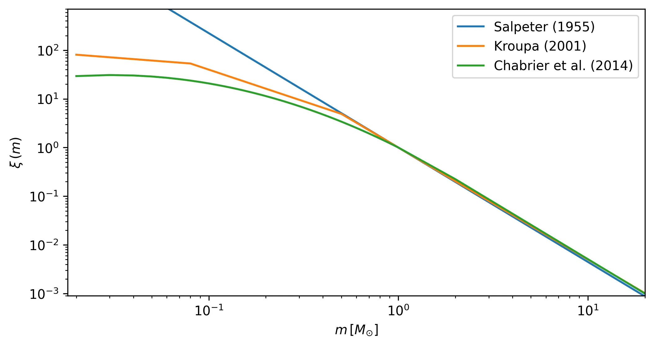
Initial mass function#
The IMF_name and max_mass arguments are used to generate random mass samples from
an IMF. To improve the performance of the code, this step is performed when the
asteca.Synthetic object is created instead of every time a new synthetic
cluster is generated. The IMF_name argument must be one of those available in
asteca.Synthetic, associated to IMFs defined in Salpeter (1955),
Kroupa (2001), and Chabrier et al. (2014) (the default value). These are
shown in the figure below:
The max_mass argument fixes the total mass value to be sampled from the IMF (hence,
it also controls the total number of synthetic stars). This
value should be large enough to allow generating as many synthetic stars as those
present in the observed cluster. The default value is \(10000\;M_{\odot}\) which
should be more than enough for the majority of clusters.
Binary systems#
The gamma argument (\(\gamma\)) defines the distribution of the mass ratio for
the binary systems. The mass ratio is the ratio of secondary masses (\(m_2\))
to primary masses (\(m_1\)) in binary systems, written as
\(q=m_2/m_1\,(<=1)\). As with the IMF, the \(q\) distribution is fixed, not
fitted, to improve the performance.
We use gamma as an argument because the \(q\) distribution is usually defined
as a power-law, where gamma or \(\gamma\) is the exponent or power:
Here, \(f(q)\) is the distribution of \(q\) (the mass-ratio) where \(\gamma(m_1)\) means that the value of \(\gamma\) depends on the primary mass of the system (this dependence is only true for the Duchene & Kraus (2013) distribution, see below).
The default selection is gamma=D&K, with D&K meaning the primary mass-dependent
distribution by Duchene & Kraus (2013) (see their Table 1 and Figure 3). The user
can also select between the two distributions by Fisher et al. (2005) (stepped
and peaked, see their Table 3) and Raghavan et al. (2010) (see their Fig 16,
left). In practice they all look somewhat similar, as shown in the figure below for a
random IMF mass sampling.
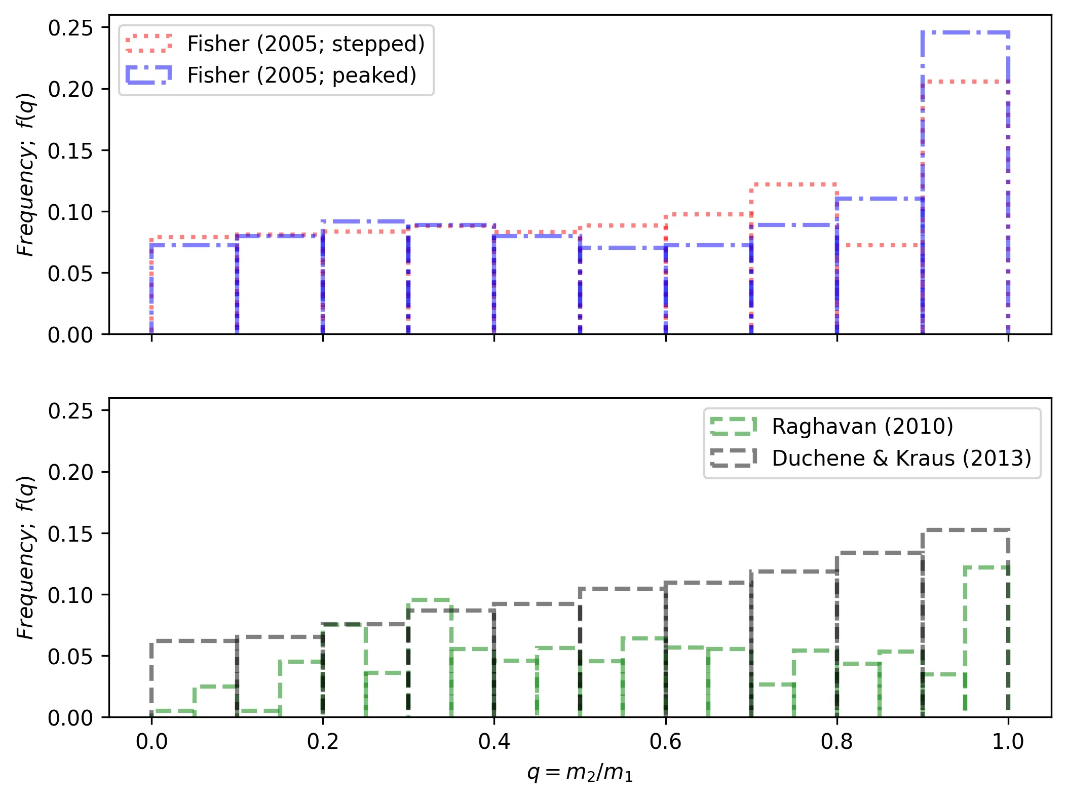
The Fisher distributions (top row) favor \(q\) values closer to unity (i.e.: secondary masses that are similar to the primary masses), while the Raghavan and Duchene & Kraus distributions (bottom row) look a bit more uniform.
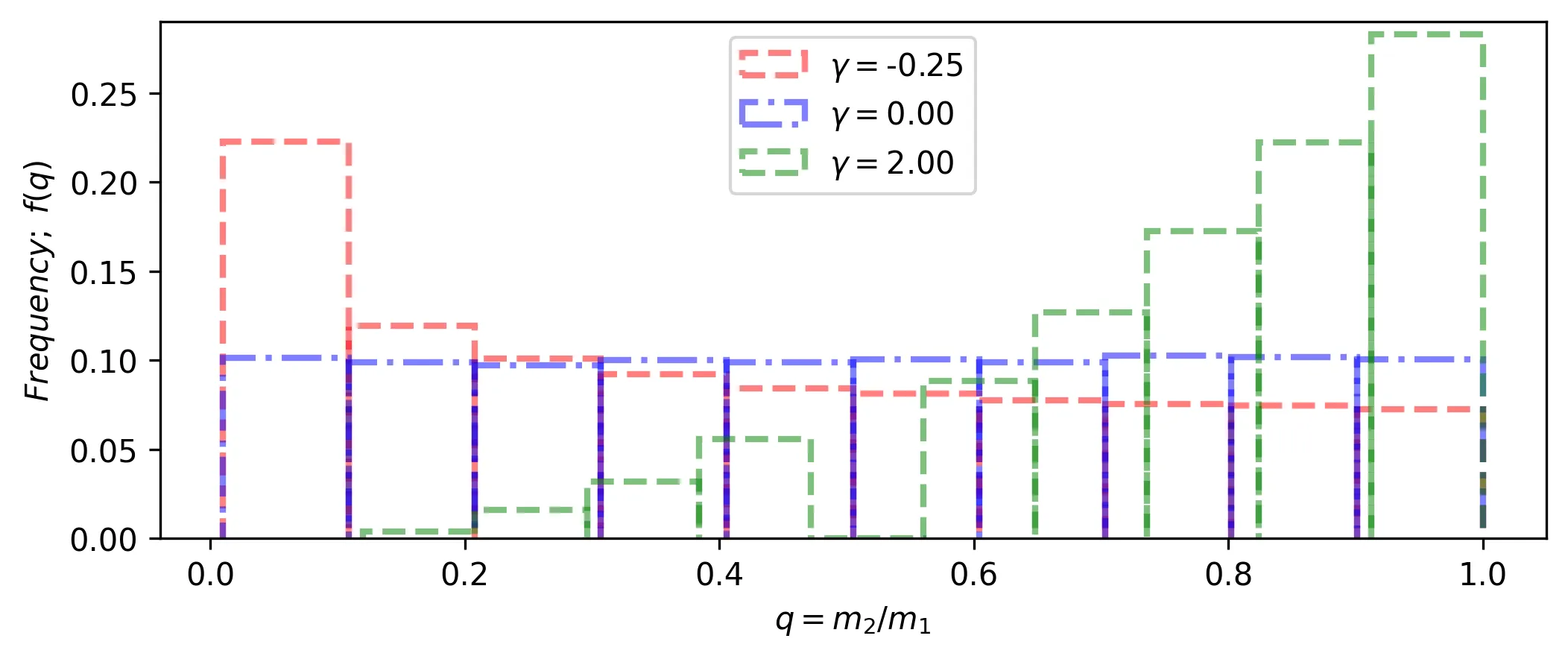
The user can also select a float value for gamma, which will be used as an
exponent in the power-law function \(f(q) \approx q^{\gamma}\). The figure below
shows this distribution for three gamma (\(\gamma\)) values, where gamma=0
means a uniform distribution.
Only the Duchene & Kraus distribution is primary-mass dependent. The Fisher and Raghavan
distributions, as well as the distributions set by the user via a float value for
gamma, are independent of mass values.
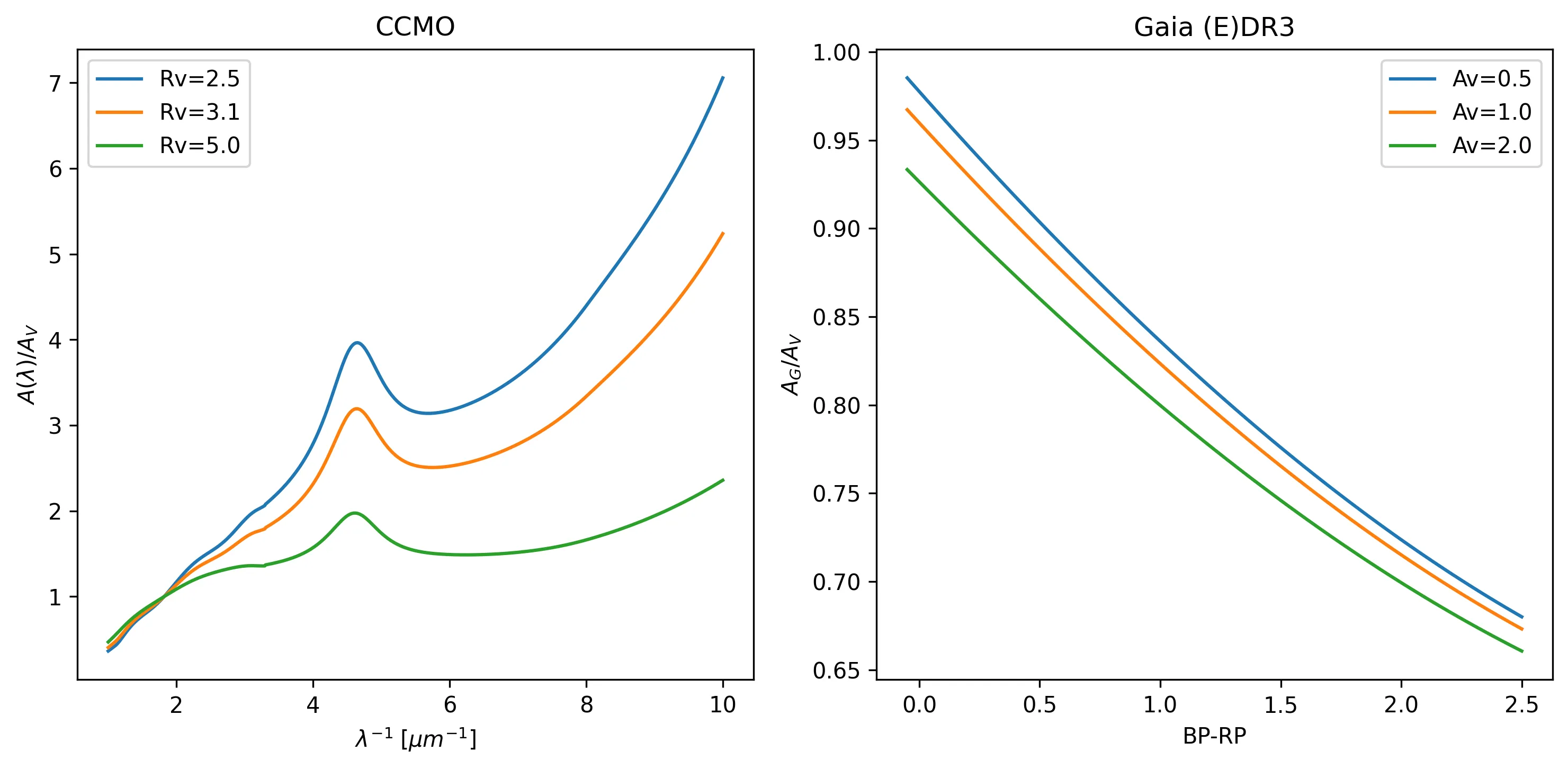
Extinction law#
An extinction law is required to transform the extinction of the photometric system
used for the observed data (the same system used for the isochrones), into the standard
total visual absorption parameter \(A_V\). This is defined by the
ext_law argument as one of either CCMO or GAIADR3.
The first one (CCMO) corresponds to the model by
Cardelli, Clayton & Mathis (1989), with updated coefficients for near-UV from
O’Donnell (1994). The second one (GAIADR3) is Gaia’s (E)DR3, color-dependent
law (main sequence), only applicable to Gaia’s photometry. If this law is selected,
ASteCA assumes that the magnitude and first color used are Gaia’s
\(G\) and \(BP-RP\) respectively.
While the CCMO law requires defining the effective lambdas for each filter
in the photometric system when defining the asteca.Isochrones object
(see Isochrones module), the GAIADR3 law does not require this data
as the extinction coefficients are already defined for Gaia’s photometry.
Important
While CCMO allows different ratio of total to selective extinction \(R_V\)
values (which means this parameter can even be fitted), GAIADR3 is to
be used with \(R_V=3.1\). Please read the online documentation and its
accompanying articles to learn more about this law’s limitations.
The figure below shows a comparison of the extinction laws implemented in ASteCA.
Left panel: the CCMO law showing the normalized extinction curve
\(A(\lambda)/A_V\) as a function of inverse wavelength for different values of
\(R_V\).
Right panel: GAIADR3 color-dependent extinction law for main-sequence stars,
applicable only to Gaia mission photometry, showing the variation of \(A_G/A_V\)
with intrinsic \(BP-RP\) color for different extinction values.
There are dedicated packages like dustapprox, dust_extinction or extinction
that can handle the extinction coefficients generation. We employ our own
implementation of the CCMO law adapted from an IDL Astronomy User’s Library
script, to increase the performance. If you want to use a different extinction model,
please drop me an email.
To load the asteca.Synthetic object with the GAIADR3 extinction
law, simply select it when instantiating the object, as follows:
# Synthetic clusters object
synthcl = asteca.Synthetic(isochs, ext_law="GAIADR3")
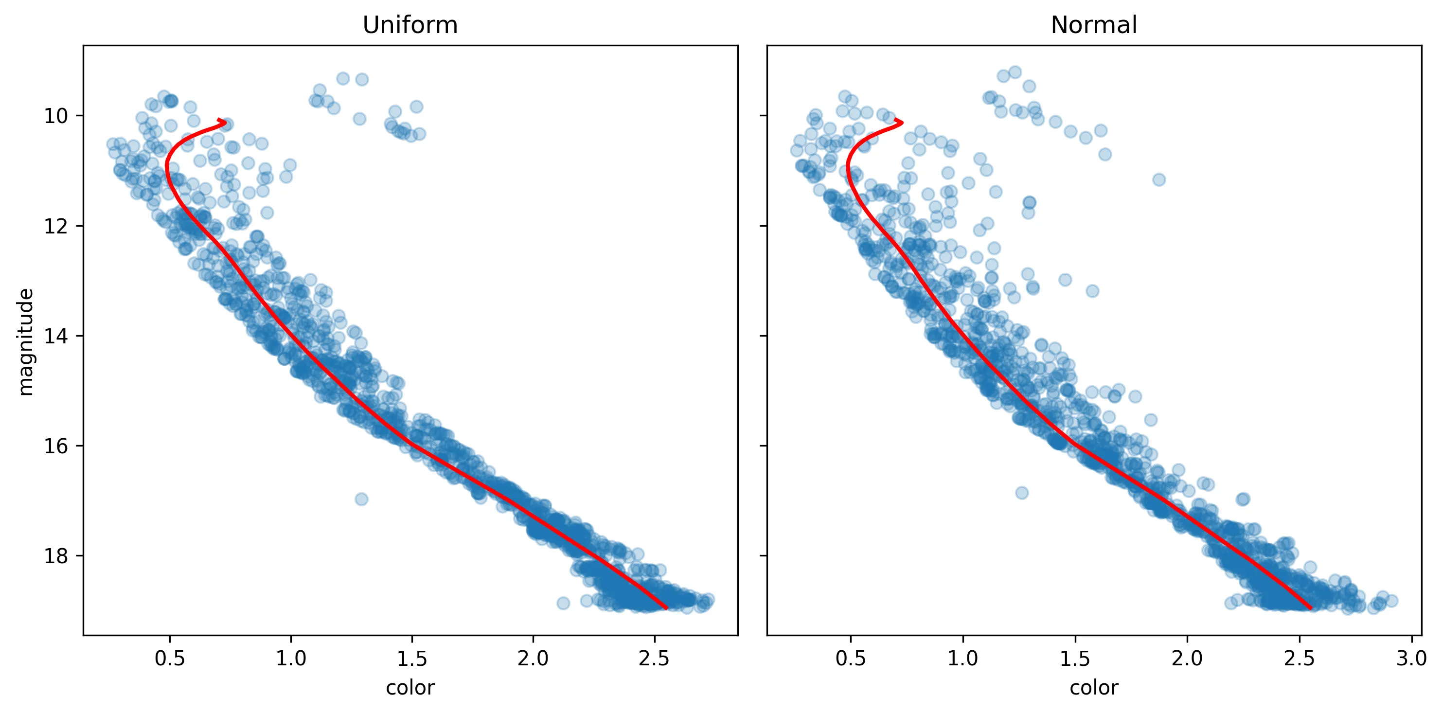
Differential reddening#
The DR_distribution argument fixes the distribution used for the differential
reddening (assuming \(DR>0\), see Section
Generating). The DR_distribution argument accepts one of two
string values: uniform (the default) or normal. These add a random amount to the
total extinction parameter \(A_V\), sampled from either a uniform or a normal
distribution (enforcing a non-negative result). The resulting reddening can be
expressed as:
where, in the uniform case:
and in the normal case:
The uniform model produces bounded, symmetric fluctuations with limited dispersion,
while the normal model yields unbounded fluctuations with heavier tails, leading to
more frequent clipping at zero and a positively skewed distribution.
The following figure shows an example of both distributions for a total extinction value of \(A_V=0.5\) and a differential reddening of \(DR=1.0\):
Calibrating#
The calibration process is applied after instantiating a asteca.Synthetic
object, named here synthcl as described in the previous section. This process
is aimed at collecting data from an observed cluster loaded in
a asteca.Cluster object (which we name here my_cluster, see
Cluster module).
The calibration is performed via the asteca.Synthetic.calibrate() method:
# Synthetic cluster calibration
synthcl.calibrate(my_cluster)
This will extract the following information from the observed cluster:
Maximum observed photometric magnitude
Number of observed stars
Distribution of photometric uncertainties
The algorithm employed by ASteCA is to simply transport the observed uncertainty values in magnitude and color(s) to the generated synthetic stars. This way no approximation to the distribution of photometric uncertainties is required.
This process is optional. The user can generate synthetic clusters
via the asteca.Synthetic.generate() method (see Generating)
without calibrating the synthcl object. In this case, the synthetic
clusters will be generated with a given number of observed stars (default value is
100 but the user can select any other value), the maximum photometric magnitude
allowed by the loaded isochrones, and no photometric uncertainties added.
The following section explains this process in more detail.
Generating#
To generate synthetic clusters the user is required to pass a dictionary with
fundamental parameters to the asteca.Synthetic.generate() method.
ASteCA currently requires eight parameters, related to the following intrinsic and
extrinsic cluster characteristics:
Extrinsic: distance modulus (
dm) and extinction related parameters (total extinctionAv, differential reddeningDR, ratio of total to selective extinctionRv)Intrinsic: metallicity (
met), age (loga), and binarity (alpha, beta)
These eight parameters are described in more depth in the following sub-sections. ASteCA also allows estimating a cluster’s total mass as well as the member stars’ masses and binary and blue straggler probabilities. This process is optional and requires fitted fundamental parameters and their STDDEVS; see Post-process parameters for more details.
An example of the dictionary of parameters used for the generation of a synthetic
cluster is shown below, fed to a previously defined synthcl object:
# Fundamental parameters dictionary
params = {
    "met": 0.0152,
    "loga": 8.0,
    "alpha": 0.0,
    "beta": 1.0,
    "Rv": 3.1,
    "DR": 0.0,
    "Av": 0.1,
    "dm": 8,
}
# Generate synthetic cluster.
synth_clust = synthcl.generate(params, N_stars=2000)
which produces a synthetic CMD similar to the one shown below. Since the
synthcl object was not calibrated against an observed cluster, no photometric
uncertainties have been added, and the maximum observed magnitude is the maximum allowed
by the loaded isochrones (the dispersion for the binary systems shown as red points is
expected):
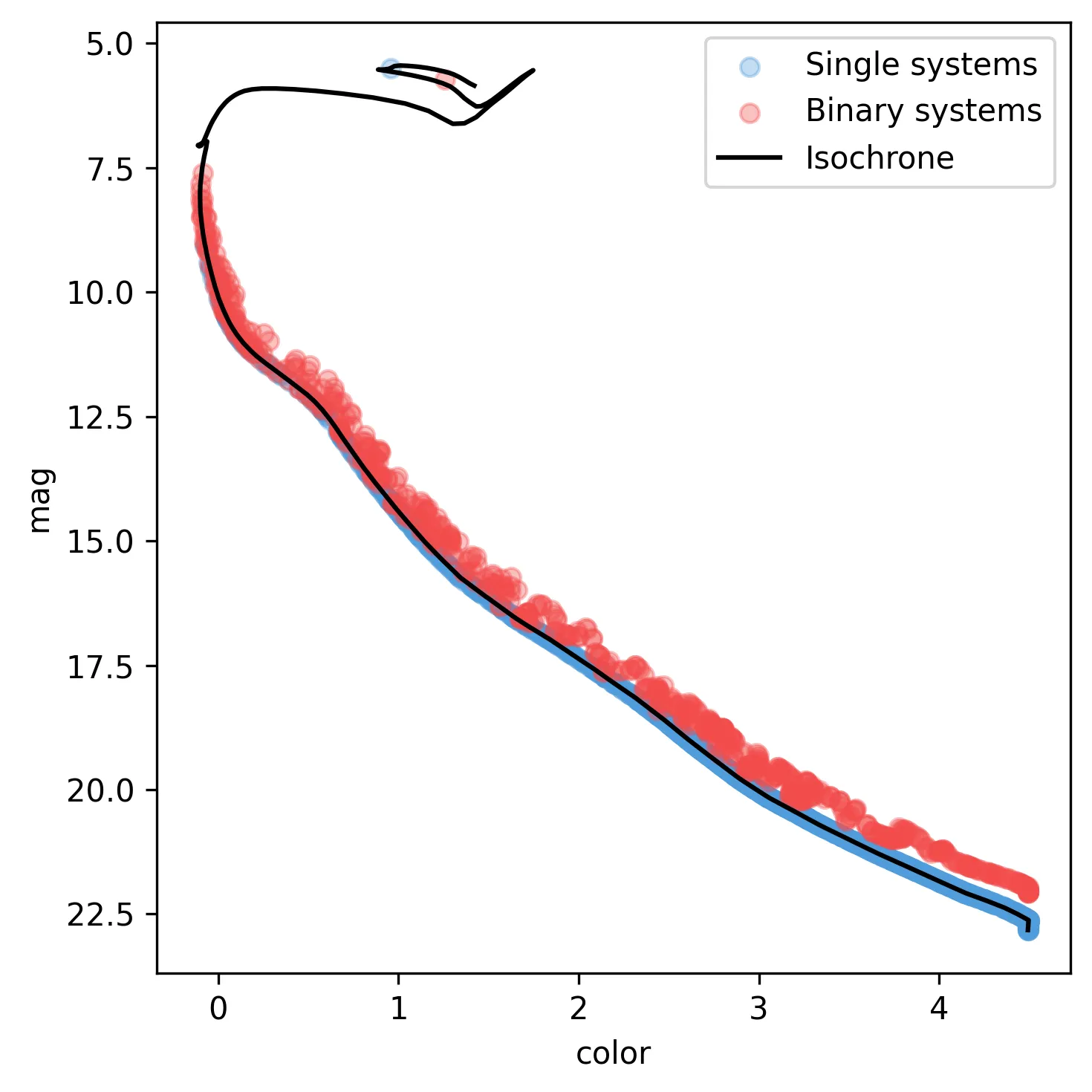
The returned synth_clust variable holds a numpy array with the synthetic
cluster data. The notebook Generate synthetic clusters contains more information and examples
on how to generate and process synthetic clusters with ASteCA.
Important
The asteca.Synthetic class includes a def_params argument with
a dictionary of default values for all the fundamental parameters. This means
that the user could call synthcl.generate() with no params dictionary,
and the method will still generate a synthetic cluster. This also allows the
user to pass a params dictionary with only a few parameters
(e.g.: params={"met": 0.02, "dm": 12.7}), and the remaining parameters will
inherit the default values. More details in Generate synthetic clusters.
Extrinsic parameters#
The four extrinsic parameters are related to two external processes affecting stellar
clusters: their distance and the extinction associated with their line of sight. The
distance is quantified through the distance modulus (dm), defined as the difference
between the apparent and absolute magnitudes, which determines the shift applied to the
cluster photometry to place the cluster at its proper distance from us.
The three remaining parameters are linked to the extinction process: the total
extinction Av, the ratio of total to selective extinction Rv, and the
differential reddening DR. The first two are related through the equation:
Finally, the differential reddening parameter DR adds random scatter to the cluster
stars affected by Av. The distribution for this scatter is controlled setting the
argument DR_distribution when the asteca.Synthetic object is
instantiated (as explained in Defining the object), which can currently be either a
uniform or a normal distribution.
Intrinsic parameters#
The four intrinsic parameters used to generate a stellar cluster are: metallicity, age, and total fraction of binary systems (controlled by two parameters).
The metallicity, met, can be modeled either as z or (logarithmic) FeH as
explained in the section Isochrones module. The age parameter, loga, is
modeled as the logarithmic age. The valid ranges for the metallicity and the logarithmic
age are inherited from the theoretical isochrone(s) loaded in the
asteca.Isochrones object.
The fraction of binary systems in a synthetic cluster is determined by the
alpha, beta parameters through the equation:
where \(P_b(m_1)\) is the probability that a star of (primary) mass \(m_1\) is part of a binary system. This equation comes from a fit to the multiplicity fraction presented in Offner et al. (2023) (see their Fig. 1 and Table 1). The multiplicity fraction values in this work are primary mass dependent, meaning that larger masses have much larger probabilities of being part of a binary (or higher order) system than low mass stars.
The values alpha=0.09, beta=0.94 produce a very reasonable fit to this multiplicity
fraction distribution:
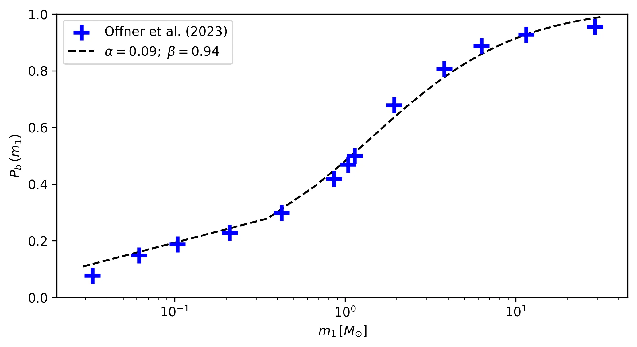
These are thus suggested as fixed values for the alpha, beta parameters. The user
can of course choose to fit either or both of them, or fix them to different values. For
example, fixing alpha=0.5, beta=0.0 would produce a synthetic cluster with
approximately 50% of binary systems, distributed uniformly across masses
(i.e.: not primary mass dependent).
Post-process parameters#
ASteCA is able to estimate extra cluster and stellar parameters, assuming that
proper fundamental parameters have been obtained for the observed cluster.
For these analyses the first step is to call the
asteca.Synthetic.calibrate() and
asteca.Synthetic.get_models() methods.
The asteca.Synthetic.calibrate() method is explained in
Calibrating, it is aimed at extracting information from the observed cluster
to generate synthetic clusters such that they are as similar as possible to the observed
cluster.
The asteca.Synthetic.get_models() method requires two input arguments:
a model dictionary, which is a dictionary of fundamental parameters assigned to
the observed cluster (however obtained), and a model_std dictionary, which contains
the uncertainties (standard deviations) associated to each parameter in model.
This method will store in the asteca.Synthetic object a number of synthetic
clusters, sampled from a normal distribution centered on the model values with
STDDEVs taken from the model_std values.
After calling these methods, we are ready to estimate:
The per-star masses (for both single and binary systems)
The per-star probability of being part of a binary system
The per-star probability of being a blue straggler (BSS)
The initial, actual, and lost masses associated to the cluster
From the per-star binary probabilities we can estimate the total binary fraction of the cluster, and from the per-star blue straggler probabilities we can estimate the total number of BSSs in the cluster.
The Post-process parameters tutorial contains examples on how to perform these analyses. The following sub-sections explain in more detail the methods used to estimate these parameters.
Stellar parameters#
ASteCA provides a simple method to assign, for each member star of your observed
cluster, its individual masses and probabilities of belonging to a binary system
and/or of being a blue straggler star (BSS). The method is called
asteca.Synthetic.stellar_parameters(), and it applies the following algorithm:
Starting from an observed cluster
Generate a synthetic cluster with some fundamental parameters
Select a given star from the observed cluster
Find the closest synthetic star (in photometric space) to this observed star
Extract from that synthetic star its primary and secondary mass values (see Stellar masses)
Classify as a binary system if the synthetic star is a binary system (see Binary fraction)
Classify as a BSS if the observed star is located inside the BSS region of the CMD (see Blue stragglers)
Repeat for all stars in the observed cluster
Repeat for
N_modelssynthetic clusters (obtained previously via theasteca.Synthetic.get_models()method)
Important
If no binary systems were generated for the synthetic clusters, i.e.: if
alpha=0, beta=0, then all the N_models secondary masses
assigned to all the observed stars will be NaN values.
At the end of this process each observed star will have N_models (synthetic)
primary and secondary masses assigned, as well as N_models classifications as
single or binary systems, and as BSS or non-BSS. Dividing these values by N_models
we can obtain the median and STDDEV of the primary and secondary masses
(m1, m1_std, m2, m2_std), as well as the binary (binar_prob) and BSS
(bss_prob) probabilities for each observed star. This information is returned in a
dictionary, e.g.:
m1          m1_std      m2          m2_std      binar_prob  bss_prob
2.097448    0.069362    0.943936    0.428501    0.955       0.00
2.448664    0.069279    0.899969    0.505402    0.880       0.00
1.144592    0.033893    0.792089    0.148655    1.000       0.00
5.128257    0.006436    0.332486    1.866812    1.000       0.00
2.013352    0.047131    0.617952    0.402121    0.925       0.00
...         ...         ...         ...         ...         ...
4.903612    0.066992    1.077981    1.053122    0.935       0.58
5.004987    0.027138    0.136899    1.547418    1.000       1.00
4.903612    0.071683    1.077981    1.111556    0.935       1.00
5.004987    0.027138    0.136899    1.547418    1.000       1.00
5.267652    0.107628    1.115867    1.133406    0.990       1.00
The sub-sections that follow explain in more detail how the stellar masses are estimated, as well as how the binary and BSS probabilities can be used to estimate the total binary fraction and the total number of BSSs in the cluster.
See the Post-process parameters tutorial for a full example on how this analysis is performed for an observed cluster.
Stellar masses#
For a given observed star i the asteca.Synthetic.stellar_parameters()
method will assign two arrays of masses of N_models length each:
observed_star_i = {
    m1_array: [0.5, 1.01, 0.32, ...],  # N_models estimates for the primary mass
    m2_array: [0.15, 0.69, NaN, ...],  # N_models estimates for the secondary mass
}
where m1_array contains the primary mass values of the closest synthetic stars to
observed_star_i in each of the N_models synthetic clusters, and m2_array
contains the secondary mass values of those same synthetic stars. If a given closest
synthetic star is a single system, then the secondary mass value assigned to
observed_star_i will be NaN.
By taking the median and the STDDEV of these two arrays, we obtain an estimate of the
primary and secondary masses (called m1 and m2 respectively), as well as their
uncertainties (m1_std and m2_std), for each observed star, i.e.:
observed_star_i = {
    m1: 0.73,  m1_std: 0.09,
    m2: 0.32,  m2_std: 0.01,
}
Note
All observed stars will have a primary and a secondary mass assigned after this
process, the secondary mass can be a NaN value. This does not mean that all
observed stars are binary systems. The user has to decide which observed stars are
binary systems and which ones are single systems. This is explained below.
For observed stars associated to single systems, only the primary mass (m1) makes
sense. On the other hand, for those observed stars better described as binary systems
(i.e: those with binar_prob>0.5), the secondary mass value estimated above
(m2) can be used to describe the total mass of the “observed binary system” as
m_tot = m1+m2.
For example, if observed_star_i has binar_prob=0.95 we can decide that it is
a binary system. Hence the primary and secondary mass values are valid and we can
use them to describe the observed binary system as:
observed_binary_star_i = {
    m1: 0.73,  m1_std: 0.09,
    m2: 0.32,  m2_std: 0.01,
}
for a total mass of the binary system of m_tot = m1 + m2 = 1.05.
If, on the other hand, observed_star_i has binar_prob=0.25 we can decide that
it is a single system. Hence the secondary mass value is of no interest and we can
ignore it. The observed star will then be described as:
observed_single_star_i = {
    m1: 0.73,  m1_std: 0.09,
}
Binary fraction#
The generation of synthetic binary systems is handled through the
alpha, beta parameters as explained in Intrinsic parameters.
The alpha, beta parameters can be fixed to given values (e.g.:
alpha=0.09, beta=0.94 to mimic the Offner et al. (2023) multiplicity fraction
distribution), or they can be fitted, to obtain values that more closely matches the
observed cluster’s binary system distribution.
There is thus no total binary fraction parameter used when generating synthetic
clusters. This parameter can be estimated via the binary system probabilities obtained
by the asteca.Synthetic.stellar_parameters() method.
The Post-process parameters tutorial shows how the median and standard deviation of the
total cluster binary fraction for an observed cluster can be computed from these
probabilities.
Blue stragglers#
The BSS region of the CMD is defined as the region above the cluster’s turn-off point and bluer than the main sequence. In ASteCA this region is defined as the region towards lower values of two points:
# The two points that define the BSS regions are defined as:
to_point_1 = [to_col + col_offset_1, to_mag + mag_offset_1]
to_point_2 = [to_col + col_offset_2, to_mag + mag_offset_2]
where the turn-off point (to_col, to_mag) is estimated by ASteCA given the
best fit isochrone. The default BSS region looks like this:
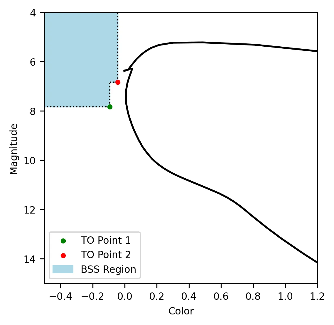
The two-point polygon allows separating the BSS region from lower mass stars in the main sequence (the TP point 1 is defined at a smaller color value than TO point 2). These stars can be affected by photometric uncertainties that make them look bluer than they actually are, thus mimicking the BSS region.
The values for the offsets (col_offset_1, mag_offset_1, col_offset_2, mag_offset_2)
can be modified by the user via the arguments of the
asteca.Synthetic.stellar_parameters() method.
Important
The current implementation assigns masses and binary probabilities to all observed stars, including those identified as probable BSSs. These values are not expected to be accurate, since the BSSs follow a younger isochrone than that used for the remaining cluster stars. The user should ignore these values until a proper implementation to handle BSSs masses and binary probabilities is implemented.
The blue straggler probability assigned to each observed star can be easily used to obtain the total number of probable BSSs in the cluster. See the Post-process parameters tutorial for an example of how this is done.
Cluster mass#
ASteCA is able to estimate different masses for an observed cluster via the
asteca.Synthetic.cluster_masses() method. This method uses the position
of the observed cluster, as well as the synthetic clusters generated
via the asteca.Synthetic.get_models() method, to estimate the initial mass of
the cluster, the actual mass, and the mass lost via stellar evolution and dynamical
effects.
The initial mass is the mass of the cluster at the moment of its formation, while the actual mass is the mass of the cluster at the present time. The difference between these two masses is the mass lost via stellar evolution and dynamical effects, which are the two main processes that cause the mass of a cluster to decrease over time. The mass lost via stellar evolution is due to the fact that stars lose mass as they evolve, while the mass lost via dynamical effects is due to the fact that stars can be ejected from the cluster due to interactions with other stars or with the tidal field of the Galaxy.
The total initial mass of a cluster, \(M_{i}\), can thus be split in several parts, as follows:
where \(M_{a}\) is the actual mass, and \(\Delta M_{evol}(t)\) & \(\Delta M_{dyn}(t)\) are the fractions of mass lost via stellar evolution and dynamical effects (or dissolution), respectively. The actual mass \(M_{a}\) can be further split as:
where \(M_{obs}\) is the observed mass and \(M_{phot}\) is the mass unobserved due to photometric effects (i.e: the low mass stars beyond the maximum observed magnitude). The observed mass \(M_{obs}\) is the sum of individual stellar masses in the observed CMD:
where \(N\) is the total number of observed stars which also includes the identified stellar binary masses.
The photometric mass \(M_{phot}\) is inferred by summing the mass that exists below the mass value associated to the maximum observed magnitude in the cluster. This requires sampling an IMF with a large mass and obtaining the ratio of the total mass \(M_{phot,s}\) to the mass of the stars brighter than the maximum observed magnitude \(M_{obs,s}\). This ratio is then applied to the observed mass \(M_{obs}\) to estimate \(M_{phot}\).
Following Lamers et al. (2005) Eq. 7, the initial mass can be estimated via:
where \(M_{a}\) is the actual mass, \(t\) is the cluster’s age, \(\mu_{\text{evol}}(Z, t)\) is the “fraction of the initial mass of the cluster that would have remained at age t, if stellar evolution would have been the only mass loss mechanism”, \({\gamma}\) is a constant, and \(t_{0}\) is “a constant that depends on the tidal field of the particular galaxy in which the cluster moves and on the ellipticity of its orbit”.
The \(\gamma\) constant is usually set to 0.62 (Boutloukos & Lamers 2003) and the \(\mu_{\text{evol}}(Z, t)\) parameter can be estimated using a 3rd degree polynomial as shown in Lamers, Baumgardt & Gieles (2010), Table B2.
The dissolution parameter \(t_0\) of a cluster is the hypothetical dissolution time-scale of a cluster of 1 \(M_{\odot}\) and is related to the disruption time \(t_{dis}\) (defined as the time when 5% of the initial number of stars remain in the cluster; Baumgardt & Makino 2003) via:
Furthermore, \(t_0\) is expected to depend on the ambient density \(\rho_{amb}\) at the location of the clusters in the Galaxy as:
where \(C_{env}\) is a constant set to 810 Myr (Lamers, Gieles & Portegies Zwart 2005), \(\epsilon\) is the eccentricity of the orbit, and \(\rho_{amb}\) is the ambient density which depends on the adopted gravitational potential field.
Following Angelo et al. (2023), ASteCA uses by default \(\epsilon=0.08\) and estimates \(\rho_{amb}\) as:
where \(\phi_B(r),\, \phi_D(\rho, z),\, \phi_H(r)\) are the bulge, disc and halo potentials, respectively (see Eqs 8, 9 and 10 of the Angelo et al. article to see how these are modeled). The user can also use a custom \(\rho_{\text{amb}}\) value, bypassing this estimation.
Plugging these values into Eq (2), we can obtain an estimate of \(M_{i}\). With this value we can then obtain \(M_{evol}\) through the \(\mu_{\text{evol}}(Z, t)\) parameter as:
Finally, the last remaining mass is the dynamical mass (mass lost via dynamical effects) which we estimate simply using Eq (1) as:
The distributions for these masses are obtained through a bootstrap process that takes the uncertainties in the fundamental parameters into account.