Synthetic clusters#

The asteca.synthetic class allows generating synthetic clusters from:

An isochrones object
A cluster object
A dictionary of fixed fundamental parameters (optional)
A dictionary of free fundamental parameters to be fitted

The handling of a synthetic object is explained in detail in the sub-sections that follow.

Defining the object#

To instantiate a synthetic object you need to pass the isochrones object previously generated, as explained in the section Loading the isochrones:

# Synthetic clusters object
synthcl = asteca.synthetic(isochs)

This example will load the theoretical isochrones into the synthetic object and perform the required initial processing. This involves sampling an initial mass function (IMF), and setting the distributions for the binary systems’ mass ratio and the differential reddening (these two last processes are optional).

The basic example above uses the default values for these three processes, but they can be modified by the user at this stage via their arguments. These arguments are (also see asteca.synthetic):

IMF_name : Initial mass function.
max_mass : Maximum total initial mass.
gamma : Distribution function for the mass ratio of the binary systems.
DR_dist : Distribution function for the differential reddening.

The IMF_name and max_mass arguments are used to generate random mass samples from a an IMF. This step is performed when the asteca.synthetic object is created instead of every time a new synthetic cluster is generated, to improve the performance of the code. The IMF_name argument must be one of those available in asteca.synthetic. Currently these are associated to the following IMFs:

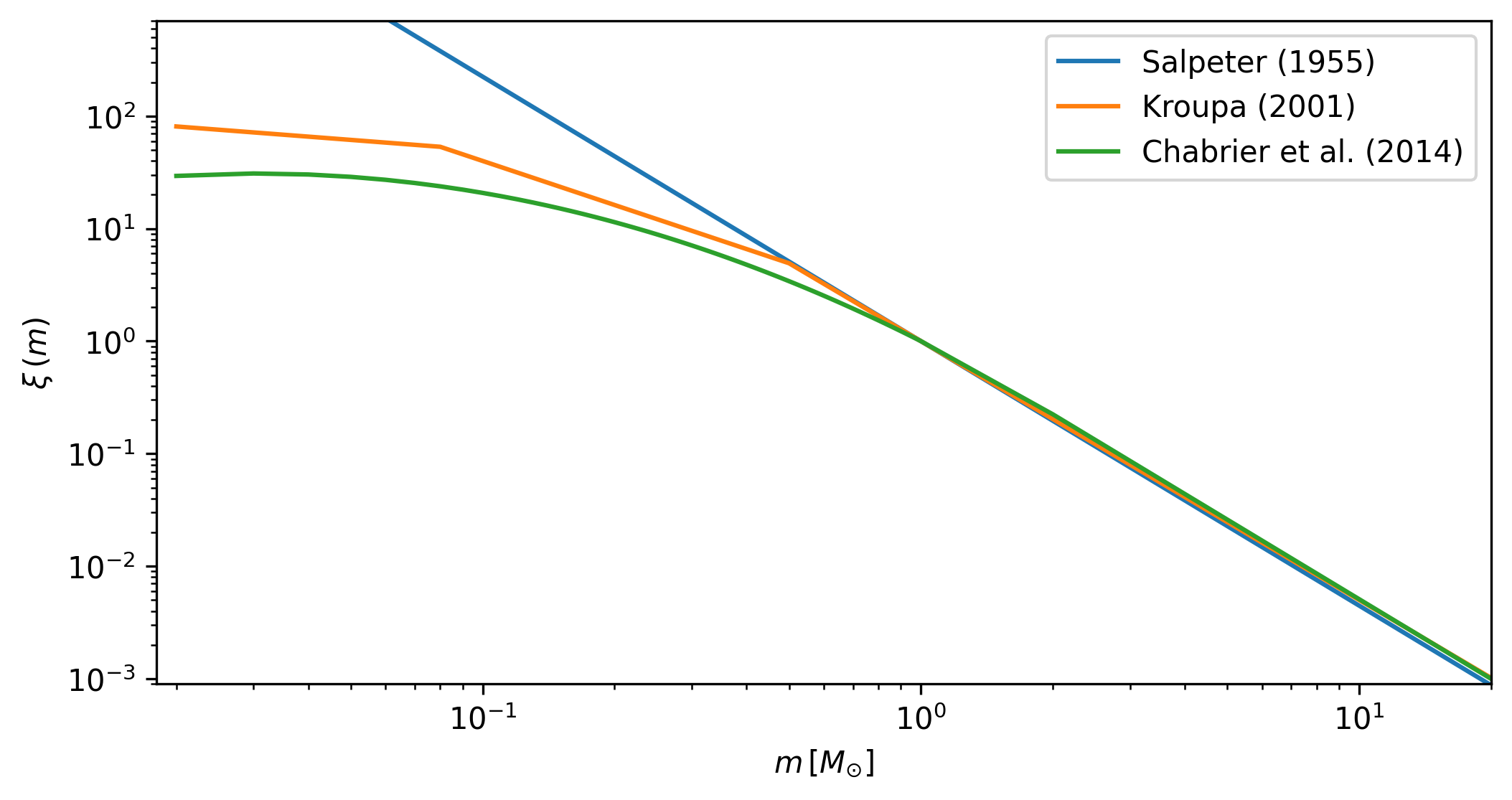
as defined in Salpeter (1995), Kroupa (2001), and Chabrier et al. (2014) (currently the default value). he max_mass argument simply fixes the total mass value to be sampled. This value is related to the number of stars in the observed cluster: it should be large enough to allow generating as many synthetic stars as those observed.

The gamma argument (\(\gamma\)) defines the distribution of the mass ratio for the binary systems. The mass ratio is the ratio of secondary masses to primary masses in binary systems. It is written as \(q=m_2/m_1\,(<=1)\) where \(m_1\) and \(m_2\) are the masses of the primary and secondary star, respectively. As with the IMF, the \(q\) distribution is fixed, not fitted, to improve the performance.

We use gamma as an argument because the \(q\) distribution is usually defined as a power-law, where gamma or \(\gamma\) is the exponent or power:

\[f(q) \approx q^{\gamma(m_1)}\]

Here, \(f(q)\) is the distribution of \(q\) (the mass-ratio) where \(\gamma(m_1)\) means that the value of \(\gamma\) depends on the primary mass of the system.

The default selection is gamma=D&K, with D&K meaning the primary mass-dependent distribution by Duchene & Kraus (2013) (see their Table 1 and Figure 3). The user can also select between the two distributions by Fisher et al. (2005) (stepped and peaked, see their Table 3) and Raghavan et al. (2010) (see their Fig 16, left). In practice they all look somewhat similar, as shown in the figure below for a random IMF mass sampling.

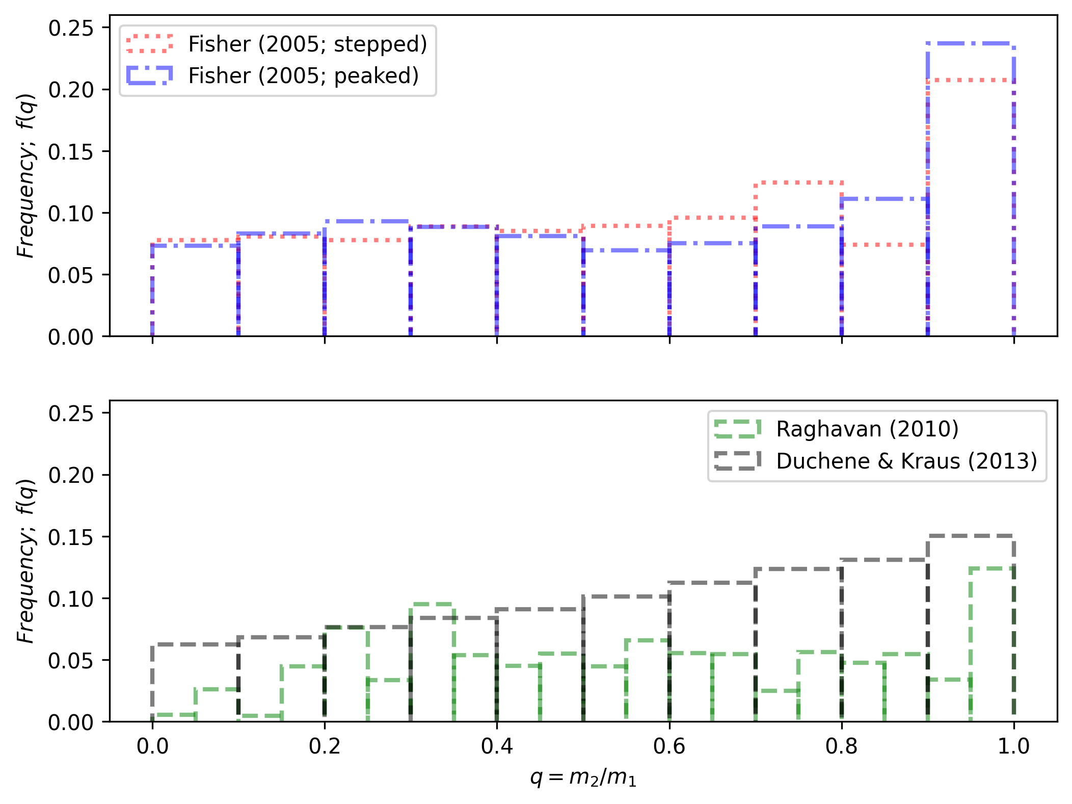
The Fisher distributions (top row) favor \(q\) values closer to unity (i.e.: secondary masses that are similar to the primary masses), while the Raghavan and Duchene & Kraus distributions (bottom row) look a bit more uniform.

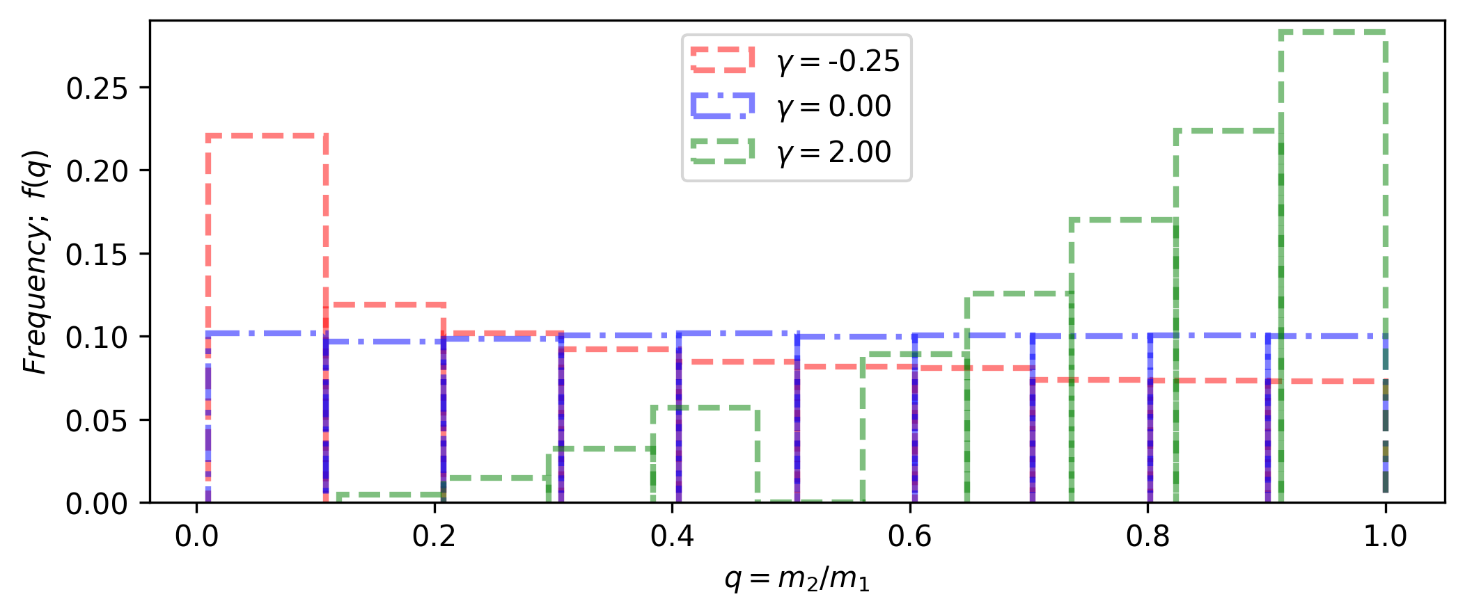
The user also select a float value for gamma, which will be used as an exponent in the power-law function \(f(q) \approx q^{\gamma}\). The figure below shows this distribution for three gamma (\(\gamma\)) values, where gamma=0 means a uniform distribution.

The DR_dist argument fixes the distribution used for the differential reddening, if this parameter is fitted to a value other than 0 (see Section Calibrating the object for more details on parameter fitting). This argument currently accepts one of two string values: uniform (the default) or normal. The differential reddening adds a random amount to the total extinction parameter Av, sampled from either a uniform or a normal distribution.

Calibrating the object#

After instantiating a synthcl object through a synthetic class (using an isochrones object and the required initial arguments: IMF, gamma, etc), we need to calibrate it with our observed cluster. This process collects required data from the cluster object (defined as my_cluster in Loading your cluster), as well as reading the fixed fundamental parameters (if any), and some initialization arguments. The basic configuration looks like this:

# Fix some model parameters
fix_params = {"alpha": 0., "beta": 1., "Rv": 3.1}
# Synthetic cluster calibration object
synthcl.calibrate(my_cluster, fix_params)

In the above example we calibrated our synthcl object with our my_cluster object defined previously, and set three fundamental parameters as fixed: alpha, beta, Rv. The meaning of these parameters is explained in the following section, we will only mention here that the fix_params dictionary is optional. If you choose not to fix any parameters, then all the fundamental parameters will be expected when calling the synthcl object to generate a synthetic cluster.

There is one more optional argument that can be used when calibrating the synthcl object: z_to_FeH. This argument is used to transform metallicity values from he default z (obtained from the loaded isochrones) to the logarithmic version FeH, and it is set to None by default. If you want to fit your synthetic cluster models using FeH instead of z, then this argument must be changed to the solar z metallicity value for the isochrones defined in the isochrones object. For example, if you are using PARSEC isochrones which have a solar metallicity of z=0.0152 (see CMD input form), then you would calibrate the synthcl object as:

synthcl.calibrate(my_cluster, fix_params, z_to_FeH=0.0152)

If this argument is not changed from its default then the z parameter will be used to generate synthetic clusters, as shown in the next section.

Generating synthetic clusters#

Once the calibration is complete, we can generate synthetic clusters by simply passing a dictionary with the fundamental parameters to be fitted to the generate() method of our synthetic object. ASteCA currently accepts eight parameters, related to three intrinsic and two extrinsic cluster characteristics:

Intrinsic: metallicity (met), age (loga), and binarity (alpha, beta)
Extrinsic: distance modulus (dm) and extinction related parameters (total extinction Av, differential reddening DR, ratio of total to selective extinction Rv)

These five cluster characteristics and its eight associated parameters are described in more depth in the following sub-sections.

Intrinsic parameters#

The valid ranges for the metallicity and logarithmic age are inherited from the theoretical isochrone(s) loaded in the isochrones object. The minimum and maximum stored values for these parameters can be obtained calling the min_max() method of our synthcl object:

met_min, met_max, loga_min, loga_max = synthcl.min_max()

The metallicity, met, can be modeled either as z or FeH as explained in the previous section. The age parameter, loga, is modeled as the logarithmic age.

The alpha, beta parameters determine the fraction of binary systems in a synthetic cluster through the equation:

\[P_b(m_1) = \alpha + \beta \times \frac{m_1}{(1.4+m_1)}\]

where \(P_b(m_1)\) is the probability that a star of (primary) mass \(m_1\) is part of a binary system. This equation comes from a fit to the multiplicity fraction presented in Offner et al. (2023) (see their Fig. 1 and Table 1). The multiplicity fraction values in this work are primary mass dependent, meaning that larger masses have much larger probabilities of being part of a binary (or higher order) system than low mass stars. The values alpha=0.09, beta=0.94 produce a very reasonable fit to this multiplicity fraction distribution:

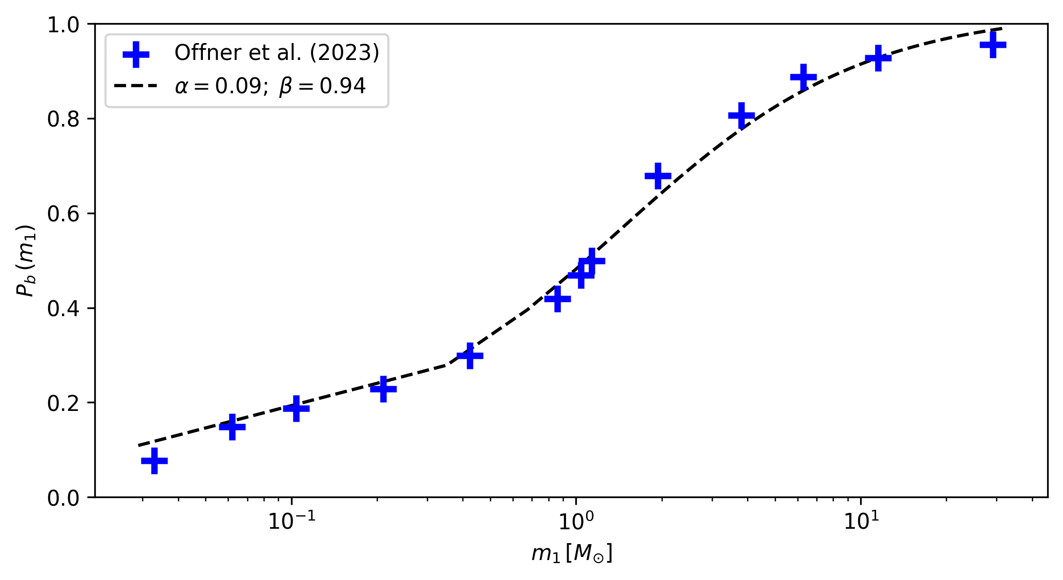
These are thus suggested as fixed values for the alpha, beta parameters. The user can of course choose to fit either or both of them, or fix them to different values. For example, fixing alpha=0.5, beta=0.0 would produce a synthetic cluster with approximately 50% of binary systems, distributed uniformly across masses (i.e.: not primary mass dependent).

Extrinsic parameters#

The extrinsic parameters are related to two external processes affecting stellar clusters: their distance and the extinction that affects them. The distance is measured by the distance modulus dm, which is the amount added to the photometric magnitude to position the cluster at the proper distance from us.

The three remaining parameters are linked to the extinction process: the total extinction Av, the ratio of total to selective extinction Rv, and the differential reddening DR.

The first two are related through the equation:

\[A_V = R_V \times E_{B-V}\]

These values are transformed to those required for the photometric systems under analysis employing the Cardelli, Clayton & Mathis (1989) model for extinction coefficients, with updated coefficients for near-UV from O’Donnell (1994). There are dedicated packages like dust_extinction that can handle this process but we use our own implementation to increase the performance. If you want to use a different extinction model, please drop me an email.

Finally, the differential reddening parameter DR adds random scatter to the cluster stars affectd by Av. The distribution for this scatter is controlled setting the argument DR_dist when the synthetic object is instantiated (as explained in Defining the object), which can currently be either a uniform or a normal distribution.

Generation#

Generating a synthetic cluster after calibrating the synthetic object simply requires calling the generate() method with a dictionary containing the parameters that were not fixed.

In the section Calibrating the object the fixed parameters were:

fix_params = {"alpha": 0., "beta": 1., "Rv": 3.1}

which means that we can generate a synthetic cluster first storing the rest of the required parameters in a dictionary (here called fit_params):

# Define model parameters
fit_params = {
    "met": 0.01,
    "loga": 9.87,
    "dm": 11.3,
    "Av": 0.15,
    "DR": 0.2,
}

and finally calling the generate() method:

# Generate the synthetic cluster
synth_clust = synthcl.generate(fit_params)

The synth_clust variable will store a numpy array of shape (Ndim, Nstars), where Ndim=2 if a single color is used and Ndim=3 if two colors are being used, and Nstars equals the number of observed stars in the cluster object (this is true ony if the max_mass argument is large enough to allow generating as many synthetic stars as those observed, otherwise fewer stars will be generated).

You can also generate a synthetic cluster passing all the available model parameters. To do this, do not pass a dictionary of fixed model parameters when calibrating the synthetic object:

# Calibrate object
synthcl.calibrate(my_cluster)

# Define all available model parameters
fit_params = {
    "met": 0.015,
    "loga": 8.75,
    "alpha": 0.0,
    "beta": 1.0,
    "dm": 8.5,
    "Av": 0.15,
    "DR": 0.0,
    "Rv": 3.1
}

# Generate the synthetic cluster
synth_clust = synthcl.generate(fit_params)

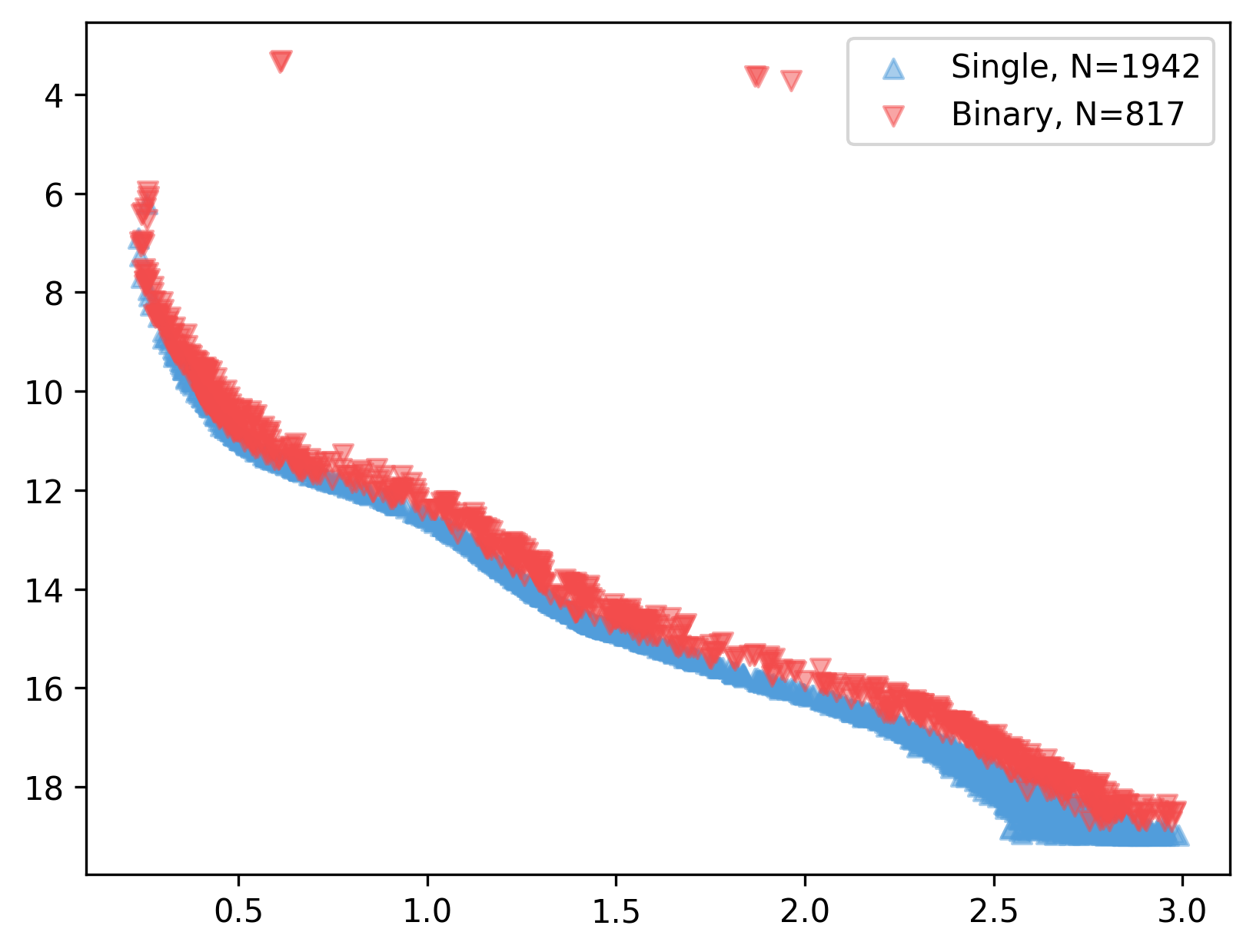
Plotting synthetic clusters#

The generated synthetic clusters can be quickly plotted using the synthplot() method:

import matplotlib.pyplot as plt

synthcl.synthplot(fit_params)
plt.show()

which will produce something like this:

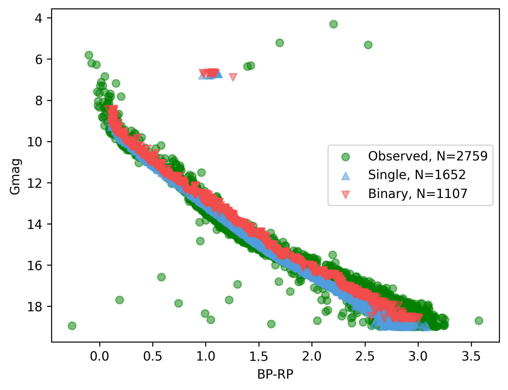
You can combine this with the clustplot() method mentioned in Loading your cluster to generate a combined CMD plot:

import matplotlib.pyplot as plt
ax = my_cluster.clustplot()
# Use the axis returned by `clustplot()`
synthcl.synthplot(fit_params, ax)
plt.show()

which produces:

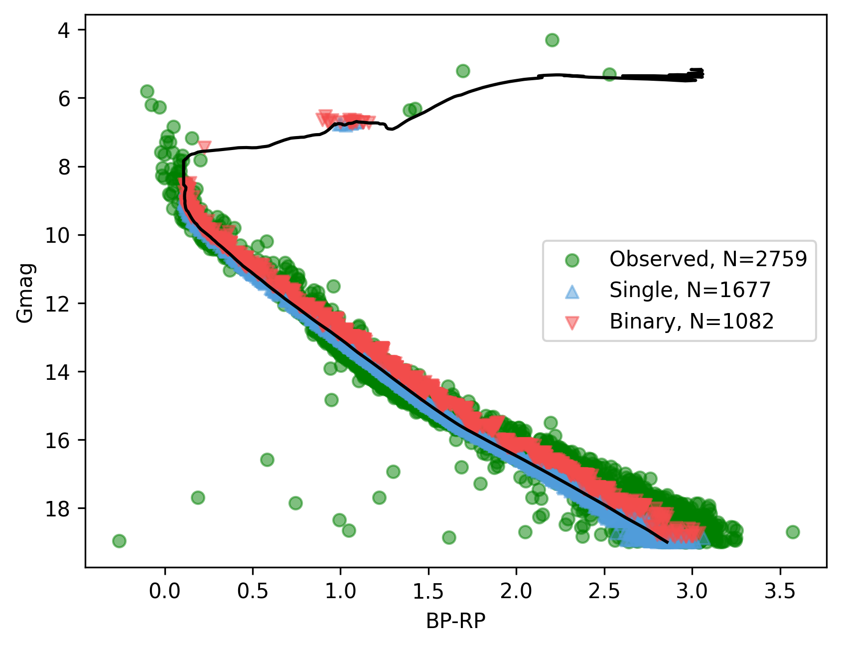
Setting the isochplot argument to True in synthplot()

synthcl.synthplot(fit_params, ax, isochplot=True)

overlays the isochrone used as a building block for the synthetic cluster:

Stellar masses and binarity#

Since the fraction of synthetic binary systems is handled through the alpha, beta parameters, there is no binary fraction parameter than can be fitted using the synthetic clusters. This needs to be generated separately, along with an estimation of the observed stars individual masses and their probability of belonging to a binary system.

This can be achieved via the masses_binary_probs() method. It requires two arguments: model which is a dictionary of parameters to be fitted (equivalent to the fit_params dictionary used to generate synthetic clusters), and a model_std dictionary which contains the uncertainties (standard deviations) associated to each parameter in the model dictionary. For example:

# Assuming alpha, beta, DR, and Rv were fixed when the object was calibrated
model = {
    "met": 0.015,
    "loga": 8.75,
    "dm": 8.5,
    "Av": 0.15,
}
model_std = {
    "met": 0.001,
    "loga": 0.2,
    "dm": 0.25,
    "Av": 0.03,
}
df_masses_bprob, binar_f = synthcl.masses_binary_probs(model, model_std)

The first variable df_masses_bprob is a pandas.Dataframe containing the columns m1, m1_std, m2, m2_std, binar_prob:

print(m1m2_bp_df)
            m1    m1_std        m2    m2_std  binar_prob
   0.544963  0.015492  0.065701  0.042717       0.025
   1.435205  0.077494  0.512087  0.276861       0.600
   0.599977  0.015769  0.133876  0.017710       0.015
   1.068667  0.051011  0.096086  0.049249       0.010
   0.772404  0.033727  0.208318  0.108373       0.175
...        ...       ...       ...       ...         ...
0.351235  0.020715  0.231247  0.045607       0.990
6.001625  0.099839  2.254647  0.863841       0.895
0.633823  0.016124       NaN       NaN       0.000
0.582850  0.016541       NaN       NaN       0.000
0.414867  0.031577       NaN       NaN       0.000

These columns represent, for each observed star in the cluster under analysis, estimates for: its primary mass (m1), its uncertainty (m1_std), its secondary mass (m2; under the assumption that this star belongs to a binary system), its uncertainty (m2_std), and its probability of being a binary system (binar_prob). If an observed star has binar_prob=0, i.e. a zero probability of being a binary system, then the mass value for its secondary star is a NaN value since no secondary star could be assigned to it.

The binar_f variable will store an array with the distribution for the total binary fraction estimate for the cluster:

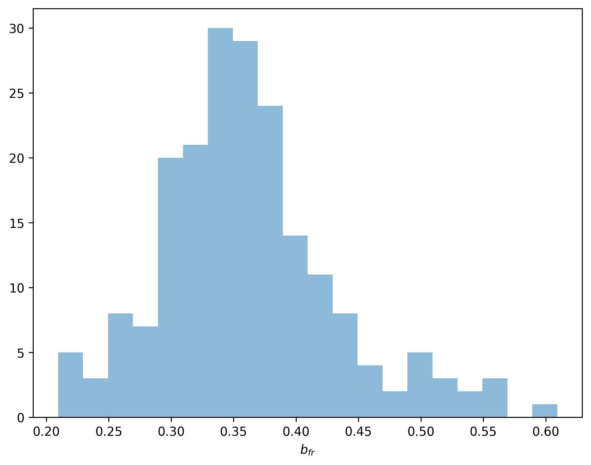
The user can obtain estimate values (e.g., mean and STDDEV) from this array, and use these as global estimates for the cluster’s binary fraction.

Synthetic clusters

Contents